MiniDynamo: A Tiny torch.compile from Scratch
When you run code under @torch.compile, a lot happens under the hood: PyTorch intercepts Python bytecode, captures a graph of tensor operations, hands that graph to an optimizing compiler, and caches the result. This article rebuilds the pieces of that system from scratch, with a small implementation that exposes the moving parts.
Note: Coding agents generated a good part of the code. I then read the implementation line by line, added tests, wrote benchmark scripts, and used the toy system to build intuition.
1. The Big Picture
PyTorch makes modeling code convenient: in a module forward() method you can use if statements, call helper functions, print for debugging, and rely on ordinary Python control flow. PyTorch calls this eager mode — each tensor operation runs the moment Python reaches it, dispatched to the device one at a time. A chain of eleven elementwise operations (like the benchmark function we will use later) means eleven kernel launches, eleven memory round-trips, and a CPU-side dispatcher between each operation. This flexibility was probably the main reason PyTorch won over TensorFlow, but it leaves performance on the table.
PyTorch 2.0 introduced torch.compile to keep the flexible Python programming model while clawing back that performance. When you wrap a function in torch.compile() and call it, PyTorch captures a graph of your tensor operations (TorchDynamo’s job), then hands that graph to an optimizing compiler (Inductor) that can fuse multiple operations into fewer kernels. Whenever the function is called again, PyTorch tries to reuse the same optimized graph, as long as the assumptions made during tracing still hold.
Why this is faster on GPUs: eager PyTorch launches one GPU kernel per operation. A fusible chain like
add → relu → mulrepeatedly reads tensors from GPU memory, writes intermediate tensors back, and pays launch overhead each time. Once Dynamo captures the whole chain as a graph, Inductor can fuse those operations into fewer kernels. In the best case, the GPU reads the data once, keeps intermediates in registers, does more work per launch, and writes the final result back once.
All of this starts with the hard part: symbolically executing arbitrary Python and PyTorch code.
The graph capture problem
Capturing a graph of tensor operations from a Python function is hard. PyTorch went through years of earlier approaches, each useful and each with painful trade-offs, before landing on TorchDynamo:
-
torch.jit.trace(2018): Run the function with example inputs and record the tensor operations that execute. Problem: it observes one execution path, not the Python program. If anifstatement takes one branch for the example inputs, the trace contains only that branch and reuses it later. Code that depends on tensor values, Python-side control flow, or input-dependent shapes can produce wrong or over-specialized graphs. -
TorchScript (
torch.jit.script, 2018): Parse Python source into a statically analyzable, typed subset of Python. This could preserve control flow in a way tracing could not. Problem: users had to write code that the TorchScript compiler understood, and real PyTorch programs often used Python features outside that subset. Many models needed code changes before they could be scripted. -
FX Tracing (
torch.fx.symbolic_trace, 2021): Execute Python withProxyobjects standing in for tensors, and record operations performed on those proxies into an FX graph. Problem: the tracer still runs ordinary Python. If Python tries to branch on a proxy value, iterate over it, or use it where a concrete value is required, tracing fails or specializes to the example-time behavior. -
Lazy Tensors: Record tensor operations at the tensor/backend level and defer execution until the result is needed. This gives the backend a graph it can optimize. Problem: Python has already run by the time those tensor ops are recorded. Lazy tensors can optimize tensor execution, but they do not solve the problem of intercepting arbitrary Python frames, understanding Python control flow, or skipping Python work on later calls.
TorchDynamo (the thing that powers torch.compile) took a different approach: it works at the bytecode level, below Python source and above the C++ dispatcher. Using PEP 523’s Frame Evaluation API, Dynamo installs a C-level hook that intercepts every Python frame before CPython’s interpreter runs it. It then walks the bytecode instructions, symbolically evaluating them to identify tensor operations and record them into an FX graph.
Calling torch.compile
-
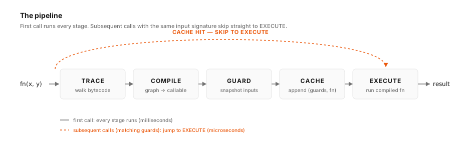
Trace: Dynamo intercepts the Python frame via PEP 523 and walks the bytecode. Tensor operations are recorded into an FX graph. Much of the surrounding Python logic is handled outside the graph: some values are evaluated concretely, some assumptions become guards, and unsupported regions can trigger graph breaks. We will see in detail what this means.
-
Compile: The FX graph is passed to a compiler backend. The default backend is Inductor, which generates Triton kernels on CUDA and C++ kernels on CPU.
-
Guard: Dynamo records the assumptions made during tracing: tensor shapes, dtypes, devices, and values of Python variables used in control flow.
-
Cache: The compiled function and its guards are stored together. On subsequent calls, if all guards pass, the compiled function is reused without re-tracing.
-
Execute: If guards pass, run the compiled function. If they fail (e.g., tensor shape changed), re-trace and compile, adding a new cache entry.
Trace once, execute many times. The first call is slow (bytecode analysis + compilation). Later calls with matching inputs skip tracing and reuse the compiled result.
What we’ll build
We will build this pipeline as a small, readable Python codebase. Our implementation, mini-dynamo, is a deliberately tiny TorchDynamo-style tracer. It captures the same core ideas while leaving out the machinery needed for arbitrary real-world PyTorch programs.
2. Architecture: The Five Components
Mini-dynamo has five pipeline stages spread across six small modules:
              fn(x, y) + example args
                      │
                      ▼
          ┌───────────────────────┐
          │   compile() decorator │ ← __init__.py (orchestrator)
          │   Manages the cache,  │   Checks guards, dispatches
          │   wires everything    │   to trace/compile/guard
          └───┬─────────┬─────┬───┘
              │         │     │
              ▼         │     ▼
  ┌──────────────────┐  │  ┌─────────────┐
  │ Symbolic          │  │  │   Guards     │ ← guards.py
  │ Interpreter       │  │  │   Shape,     │   Boolean checks on
  │                   │  │  │   dtype,     │   input metadata
  │ Walks bytecodes,  │  │  │   device     │
  │ manipulates       │  │  └─────────────┘
  │ VariableTrackers  │  │
  │ on a stack,       │  │
  │ builds the Graph  │  │
  └────────┬──────────┘  │
           │             │
     ┌─────┘             │
     ▼                   ▼
  ┌──────────┐    ┌──────────────┐
  │  Graph   │───▶│  Compiler    │ ← compiler.py
  │  (IR)    │    │  Backend     │   Graph → Python source
  │          │    │              │   → exec() → callable
  └──────────┘    └──────────────┘
   graph.py         examples/ → Inductor
The package backend in mini_dynamo/compiler.py only implements the Python and JIT paths exposed by @mini_dynamo.compile. The Inductor path appears later as an example script that converts the mini graph to FX, lowers it to ATen, and calls a private Inductor entry point.
The table maps each component to its TorchDynamo counterpart:
| Mini-dynamo | Real TorchDynamo | Role |
|---|---|---|
symbolic_interpreter.py | InstructionTranslator (~5,000 lines in symbolic_convert.py) | Walk bytecodes, build the graph. The heart of the system. |
variable_tracker.py | VariableTracker hierarchy (200+ subclasses across ~20 files) | Symbolic values on the interpreter’s stack. Tell the interpreter what kind of thing each value is (tensor? constant? torch function?) so it can decide whether to record a graph node or evaluate concretely. |
graph.py | torch.fx.Graph + torch.fx.Node | The computation graph IR. A flat list of nodes, each describing one operation. This is the output of tracing and the input to compilation. |
compiler.py | Compiler backends (Inductor, etc.) | Takes a finished graph and produces a callable. Our simple backend generates Python source with pre-resolved names in an exec() namespace. Real Inductor generates Triton GPU kernels and C++ CPU kernels. The later Inductor integration example adds a small converter from our graph format to FX Graphs. |
guards.py | torch._dynamo.guards (C-accelerated) | Boolean predicates that encode the assumptions made during tracing. If guards pass on new inputs, the cached compiled function can be reused. |
__init__.py | torch._dynamo.convert_frame | The orchestrator. Manages the guard-cache loop: check guards → hit? run cached fn. Miss? trace → compile → guard → cache. |
Two components deserve special attention because their roles are easy to confuse:
The Graph is the output. It is a pure data structure: a list of nodes describing which tensor operations to perform. It has no logic and no execution semantics. After tracing, the compiler receives it as a recipe.
VariableTrackers are the process. They are the symbolic values that live on the interpreter’s stack during tracing. They tell the interpreter what type of thing each value is, so it can decide what to do with each bytecode instruction. When tracing finishes, the interpreter throws them away. They are scaffolding for the graph, not part of the final product.
We need both because CPython’s bytecodes are untyped. When the interpreter sees BINARY_ADD, it doesn’t know if it’s adding two tensors (→ record torch.add in the graph) or two integers (→ just compute the result). VariableTrackers carry the type information that lets it make this decision. The Graph records the decisions that were made.
3. CPython Is a Stack Machine
To understand our symbolic interpreter, you need one fact about CPython: it’s a stack-based virtual machine. Every Python function compiles to a sequence of bytecode instructions that manipulate a value stack and a locals array.
For z = x + y, CPython emits:
| Instruction | Stack (after) | Effect |
|---|---|---|
LOAD_FAST x | [x] | Push local variable x |
LOAD_FAST y | [x, y] | Push local variable y |
BINARY_ADD | [x+y] | Pop two, push their sum |
STORE_FAST z | [] | Pop and store in local z |
Our symbolic interpreter mirrors this exactly – same stack, same locals, same dispatch loop. The only difference: instead of real Python values, the stack holds symbolic wrappers that record operations into a graph.
4. VariableTrackers: The Symbolic Values
Every value in our interpreter is a VariableTracker: “I’m not a real value. I’m a description of a value that will exist at runtime.”
We need exactly four types:
TensorVariable
The most important type. It holds a graph node (its identity in the computation graph) and an example value (a real tensor with the same shape/dtype/device, used for metadata propagation).
class TensorVariable(VariableTracker):
    def __init__(self, node, example_value):
        self.node = node              # Graph Node that produces this tensor
        self.example_value = example_value  # Real tensor for shape tracking
When the interpreter sees x + y where both are TensorVariables, it doesn’t compute the runtime result that the user asked for. Instead, it:
- Creates a new
Nodein the graph:call_function(torch.add, (x.node, y.node)) - Computes an example output for metadata propagation:
torch.add(x.example_value, y.example_value) - Returns
TensorVariable(new_node, example_output)
The example value flows forward through every operation, so at any point during tracing, we know the exact shape, dtype, and device of every intermediate tensor. We are still running individual example tensor ops during tracing to propagate metadata, but the output of tracing is the graph, not the eager result of the original function.
ConstantVariable
A value fully known at trace time: the 2 in x * 2, a dtype like torch.float32, a shape tuple. Constants don’t become graph nodes – they’re inlined directly into the operations that use them.
class ConstantVariable(VariableTracker):
    def __init__(self, value):
        self.value = value  # The actual Python value
TorchVariable
A reference to the torch module or one of its functions. When the interpreter encounters LOAD_GLOBAL torch, it pushes TorchVariable(torch). When it then encounters LOAD_ATTR relu, it resolves torch.relu and pushes TorchVariable(torch.relu).
MethodVariable
A bound tensor method like x.sum. Created when the interpreter accesses a method on a TensorVariable. It remembers which tensor and which method, so when called, it can record the correct graph node.
5. The Graph IR
As the interpreter runs, it records operations into a Graph – an ordered list of Node objects that form a DAG of the computation. This is a simplified version of torch.fx.Graph.
Each Node has four key fields:
class Node:
    name: str       # Unique identifier, e.g. "add_0", "x"
    op: str         # One of: "placeholder", "call_function", "call_method", "output"
    target: Any     # What to call (e.g., torch.add) or method name (e.g., "sum")
    args: tuple     # Positional arguments -- can reference other Nodes
Nodes come in four flavors:
op | Meaning | Example |
|---|---|---|
placeholder | Function input | x = placeholder |
call_function | A function call on tensors | add_0 = torch.add(x, y) |
call_method | A method call on a tensor | sum_0 = add_0.sum() |
output | The return value | return sum_0 |
For the function:
def fn(x, y):
    z = x + y
    w = z * 2
    return w.sum()
The captured graph is:
Graph:
  x = placeholder
  y = placeholder
  add_0 = torch.add(x, y)
  mul_0 = torch.mul(add_0, 2)
  sum_0 = mul_0.sum()
  return sum_0
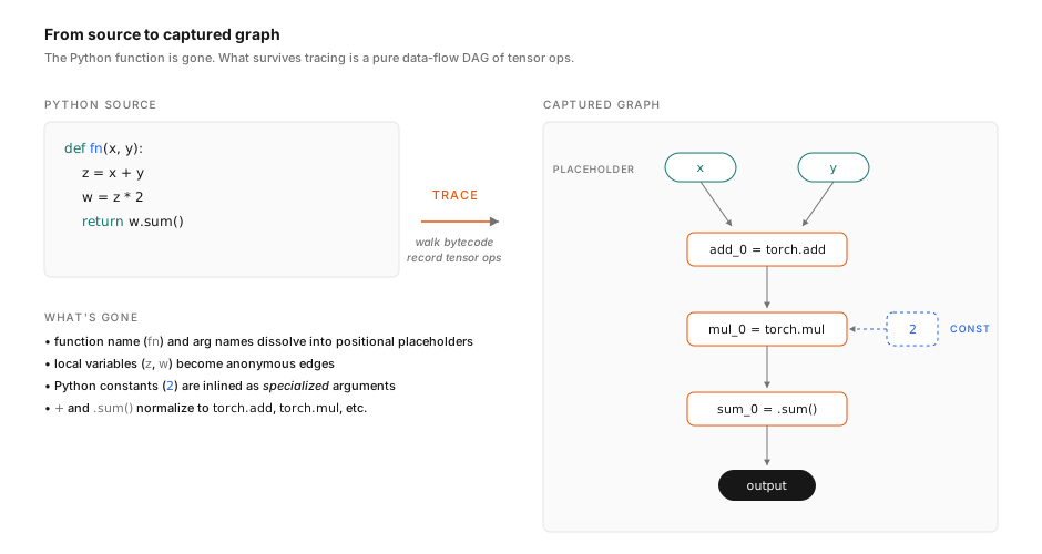
Notice the 2 in torch.mul(add_0, 2) – it’s a plain Python integer, not a Node. Constants are inlined into the args of the operations that consume them.
6. The Symbolic Interpreter
The SymbolicInterpreter ties the previous pieces together. It reads bytecode, manipulates VariableTrackers on a stack, and writes nodes into the Graph. Everything else feeds into this loop or consumes its output.
When you run a Python function normally, CPython walks the bytecode and executes each instruction on real objects: integers get added, tensors get multiplied, methods get invoked. We use the same bytecode and stack discipline, but we care about the shape of the computation rather than the user-facing return value. We re-implement enough of CPython’s interpreter to produce a graph.
Two Interpreters in Parallel
Picture two interpreters running side by side on the same bytecode, one real and one symbolic:
| CPython’s interpreter | Our symbolic interpreter | |
|---|---|---|
| Stack holds | Real Python objects | VariableTrackers |
| Locals hold | Real values | VariableTrackers |
BINARY_ADD on two tensors | Calls torch.add, produces a new tensor | Records torch.add(x, y) in the graph, pushes a new TensorVariable wrapping that node |
BINARY_ADD on two ints | Computes a + b | Computes a + b; constants are evaluated concretely |
CALL_METHOD x.sum() | Invokes the bound method | Records x.sum() in the graph |
| Unsupported opcode | Executes it | Raises NotImplementedError |
| Final output | A return value | A finished Graph |
CPython operates on values; mini-dynamo operates on descriptions of values. At every bytecode step, the symbolic interpreter makes one decision: record this operation into the graph, or evaluate it concretely on constants and metadata we already know. Repeating that decision across instructions produces the captured graph.
The Three Pieces of State
Just like CPython, our interpreter carries three pieces of state through its run:
-
self.stack: a list ofVariableTrackers.LOAD_*opcodes push to it;BINARY_*,CALL_*,STORE_*, and the rest consume it. -
self.locals: a dict mapping variable names toVariableTrackers. It starts with the function arguments and changes onSTORE_FAST. -
self.graph: theGraphbeing built. It grows each time a tensor operation gets recorded.
Everything the interpreter does is a transformation of these three. If you snapshotted them after every instruction, you’d have a complete movie of the trace.
Correspondence to Real Dynamo
Our SymbolicInterpreter is the direct analogue of TorchDynamo’s InstructionTranslator (in torch/_dynamo/symbolic_convert.py). The two share the same skeleton: a value stack, a locals dict, an FX-style graph being mutated, and one handler per opcode. The differences are in scope, not in kind:
- Real Dynamo handles ~160 opcodes including jumps, comparisons, exceptions, closures, and generator machinery. We handle a small straight-line subset.
- Real Dynamo inline-traces into called functions. When
fn()callshelper(), the tracer recursively walks the callee’s bytecode too — during tracing,helper’s frame never actually runs — producing a single unified graph. Our walker only sees top-level bytecode; if it records a helper call at all, it records it as an opaque callable rather than looking inside. - Real Dynamo emits guards on-the-fly as it makes assumptions (e.g. “I looked at
x.shape[0]and treated it as32, so guard on that”). We emit guards after tracing, from the example inputs. - Real Dynamo can break the graph when it hits something unsupported: compile what it has so far, let the hard part run in plain Python, and resume tracing after. Our interpreter halts with
NotImplementedError.
From here, we follow the walker from initialization through dispatch, then trace one example and finish with the call-dispatch logic that decides whether a call becomes a graph node or a concrete Python call.
Initialization
When we begin tracing fn(x, y), we create a SymbolicInterpreter with:
- A fresh
Graph - An empty
stack -
localspopulated withTensorVariableplaceholders for each tensor argument
def __init__(self, fn, example_args):
    self.fn = fn
    self.graph = Graph()
    self.stack = []     # Mirrors CPython's value stack, but holds VariableTrackers
    self.locals = {}    # Mirrors CPython's locals: name -> VariableTracker
    self.globals = fn.__globals__  # Needed later for LOAD_GLOBAL (e.g. `torch`)

    # fn.__code__ is the compiled CPython code object behind a function.
    # co_varnames is the tuple of *all* local names; the first co_argcount of
    # them are the declared parameters, in order. So this slice gives us just
    # the parameter names without pulling in interior locals.
    code = fn.__code__
    arg_names = code.co_varnames[:code.co_argcount]

    # Seed the locals dict with one tracker per argument:
    #   - tensors enter the graph as `placeholder` nodes (they're the inputs
    #     downstream nodes will reference);
    #   - non-tensors stay as concrete ConstantVariables, so the interpreter
    #     can use their actual Python value during tracing (e.g. literal
    #     arithmetic, shape tuples, dtype objects). The public decorator
    #     intentionally rejects non-tensor runtime arguments.
    for name, example in zip(arg_names, example_args):
        if isinstance(example, torch.Tensor):
            node = self.graph.placeholder(name)
            self.locals[name] = TensorVariable(node, example)
        else:
            self.locals[name] = ConstantVariable(example)
The Main Loop
The interpreter fetches instructions one by one and dispatches to handler methods:
def run(self):
    # dis.get_instructions decodes the function's bytecode into a flat list
    # of Instruction records: the same data CPython would dispatch on
    # internally. Each record knows its opname (e.g. "LOAD_FAST"), its
    # argument value, and where it sits in the bytecode.
    instructions = list(dis.get_instructions(self.fn))
    for inst in instructions:
        # One handler method per opcode, conventionally named op_<OPNAME>
        # (e.g. op_LOAD_FAST, op_BINARY_ADD). This is the same trick CPython's
        # ceval.c uses, spelled in Python via attribute lookup. Anything
        # we haven't implemented falls through to NotImplementedError rather
        # than silently producing a wrong graph.
        handler = getattr(self, f"op_{inst.opname}", None)
        if handler is None:
            raise NotImplementedError(f"Unsupported bytecode: {inst.opname}")
        handler(inst)
    return self.graph
Walking Through an Example
Trace fn(x, y), where fn computes z = x + y; w = z * 2; return w.sum(). The first four instructions show bytecode, stack, and graph evolving in lockstep:
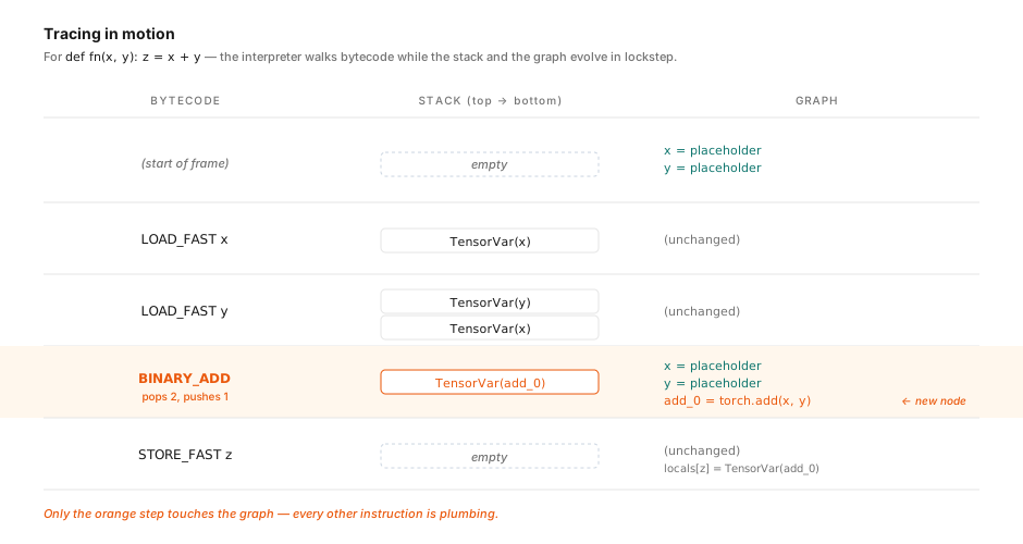
The full trace, including the multiplication and the method call:
| Step | Instruction | Stack | Graph (new node) |
|---|---|---|---|
| 1 | LOAD_FAST x | [TensorVar(x)] | – |
| 2 | LOAD_FAST y | [TensorVar(x), TensorVar(y)] | – |
| 3 | BINARY_ADD | [TensorVar(add_0)] | add_0 = torch.add(x, y) |
| 4 | STORE_FAST z | [] | – |
| 5 | LOAD_FAST z | [TensorVar(add_0)] | – |
| 6 | LOAD_CONST 2 | [TensorVar(add_0), ConstVar(2)] | – |
| 7 | BINARY_MULTIPLY | [TensorVar(mul_0)] | mul_0 = torch.mul(add_0, 2) |
| 8 | STORE_FAST w | [] | – |
| 9 | LOAD_FAST w | [TensorVar(mul_0)] | – |
| 10 | LOAD_METHOD sum | [MethodVar(mul_0, "sum")] | – |
| 11 | CALL_METHOD 0 | [TensorVar(sum_0)] | sum_0 = mul_0.sum() |
| 12 | RETURN_VALUE | [] | return sum_0 |
Notice three details:
Steps 3 and 7 – when a binary operation involves a TensorVariable, the interpreter records a torch.add or torch.mul node in the graph and pushes a new TensorVariable wrapping that node. The constant 2 is passed directly into the node’s args.
Step 10 – LOAD_METHOD sum on a TensorVariable produces a MethodVariable, not a graph node. The method has been looked up, not called. Step 11 creates the graph node when CALL_METHOD executes it.
Step 12 – RETURN_VALUE marks the output. The graph is now complete.
The Call Dispatch Logic
The most interesting handler is _handle_call, which decides what to do when a function or method is called:
def _handle_call(self, fn, args):
    # Known torch function with tensor args? → Record graph node.
    if isinstance(fn, TorchVariable) and fn.value in SUPPORTED_TORCH_FUNCTIONS:
        return self._call_torch_function(fn.value, args)

    # Tensor method (x.sum, x.reshape)? → Record graph node.
    if isinstance(fn, MethodVariable):
        return self._call_tensor_method(fn, args)

    # Unknown callable with tensor args? → Try tracing it anyway.
    if isinstance(fn, TorchVariable) and callable(fn.value):
        has_tensors = any(isinstance(a, TensorVariable) for a in args)
        if has_tensors:
            return self._call_torch_function(fn.value, args)
        else:
            concrete_args = [self._to_concrete(a) for a in args]
            return self._wrap_result(fn.value(*concrete_args))

    # Pure Python on constants (int, len, etc.)? → Evaluate directly.
    if isinstance(fn, ConstantVariable) and callable(fn.value):
        concrete_args = [self._to_concrete(a) for a in args]
        return self._wrap_result(fn.value(*concrete_args))

    raise RuntimeError(f"Don't know how to call {type(fn).__name__}")
The design has three paths: known tensor operations are traced; opaque global callables with tensor inputs can be recorded as call_function nodes; supported pure-Python work on constants is evaluated. Mini-dynamo still raises outside that narrow subset, especially for unsupported bytecodes, keyword calls, and non-tensor returns. Real TorchDynamo can guard on Python values, rewrite bytecode, and resume after graph breaks. A graph break is Dynamo’s escape hatch for the “don’t know how to handle this” case: it compiles the graph it has built so far, hands control back to the regular Python interpreter to run the unsupported bit (a print, an unusual data structure, a call into a C extension), and then starts a fresh trace from the next instruction. A single Python function can become several compiled graphs stitched together with plain eager code in between.
7. The Compiler Backend
The graph is now a clean IR of tensor operations. The compiler’s job is to turn it into a callable. In torch.compile, this is where the graph gets handed to Inductor for kernel fusion, the step that produces the speedup. Our educational backend does something smaller. It generates a plain Python function that re-dispatches to the same torch ops as the original, one at a time, with function lookups pre-resolved into the generated function’s namespace. It proves we captured the graph correctly and produces a standalone callable you could feed to real Inductor later. It does not create speedups.
What the compiler generates
Our compiler walks the graph and generates a Python function with all function references pre-resolved in the exec() namespace:
# Generated code for many_ops(x, y):
def compiled_fn(x, y):
    add_0 = __fn_add_0(x, y)       # __fn_add_0 = torch.add (in exec namespace)
    mul_0 = __fn_mul_0(add_0, 2)   # __fn_mul_0 = torch.mul (in exec namespace)
    sub_0 = __fn_sub_0(mul_0, x)   # __fn_sub_0 = torch.sub (in exec namespace)
    ...
    return sum_0
Each __fn_* variable is resolved from the custom namespace we pass to exec(), avoiding the LOAD_GLOBAL torch + LOAD_ATTR add pair in the original. That sounds like an optimization, but it saves very little. CPython’s bytecode dispatch runs on the order of tens of nanoseconds per instruction, while a single eager PyTorch op on the GPU spends microseconds in the C++ dispatcher, more microseconds launching the kernel, and then whatever the kernel itself takes. Skipping one LOAD_GLOBAL + LOAD_ATTR pair per op saves at most a tiny fraction of the smallest of those costs. This step exists to produce a clean, self-contained callable that reproduces the graph. An optimizing backend like Inductor expects that kind of graph-shaped callable as input, and it gives us a useful sanity check that our tracer matched the original function.
Code Generation
The compiler walks the graph and emits one line of Python per node:
def compile_graph(graph):
    # Graph placeholders become the parameters of the generated function,
    # in the same order they appeared in the original `fn`.
    param_names = [n.name for n in graph.inputs]
    signature = ", ".join(param_names)

    body_lines = []
    # `closure_vars` ends up as the globals dict for the exec()'d function.
    # Stashing the actual callables (torch.add, torch.mul, …) in here lets
    # generated code refer to them as plain names — no LOAD_GLOBAL + LOAD_ATTR
    # pair on every call.
    closure_vars = {}

    for node in graph.nodes:
        if node.op == "placeholder":
            continue  # Already covered by the function signature above.
        elif node.op == "call_function":
            # Give this op a unique closure key, stash its target callable,
            # and emit a single line that invokes it.
            closure_key = f"__fn_{node.name}"
            closure_vars[closure_key] = node.target
            args_str = _format_call_args(node.args)
            body_lines.append(f"    {node.name} = {closure_key}({args_str})")
        elif node.op == "call_method":
            # Methods are dispatched on the receiver, so there's no callable
            # to stash in the exec namespace. We write `<self>.<method>(...)`.
            self_name = _arg_to_str(node.args[0])
            rest_args = _format_call_args(node.args[1:])
            body_lines.append(f"    {node.name} = {self_name}.{node.target}({rest_args})")
        elif node.op == "output":
            body_lines.append(f"    return {_arg_to_str(node.args[0])}")

    source = f"def compiled_fn({signature}):\n" + "\n".join(body_lines)
    # Two-step materialization. `compile()` (Python builtin, not ours) turns
    # the source string into a code object; `exec()` runs that code with
    # `closure_vars` as its globals. The side effect is that `compiled_fn`
    # is now defined inside `closure_vars`, ready to be pulled back out.
    code = compile(source, "<mini-dynamo-compiled>", "exec")
    exec(code, closure_vars)
    return closure_vars["compiled_fn"], source
The exec() call creates the function in a namespace that contains the pre-resolved torch functions. This string-codegen trick belongs to our educational backend. Real TorchDynamo’s default path produces FX graphs and hands them to backends such as Inductor; it does not rely on this tiny Python source generator for performance.
The JIT Backend
For an additional step, we can trace the generated Python function with torch.jit.trace to get a TorchScript function:
def compile_graph_jit(graph, example_inputs):
    # First, produce our usual Python source via compile_graph(). Then hand
    # that callable to torch.jit.trace, which re-records it as a single
    # TorchScript graph by running it once with the example inputs. The
    # result is a function where Python drops out of the per-op loop,
    # but each op still launches its own kernel; nothing is fused.
    compiled_fn, source = compile_graph(graph)
    traced_fn = torch.jit.trace(compiled_fn, example_inputs)
    return traced_fn, source
The result is a TorchScript function where the entire graph executes as a single C++ call, with no Python interpreter between operations. Each operation still launches a separate kernel. There is no kernel fusion, so this is not the same optimization path as Inductor; in small GPU microbenchmarks it can still help by reducing Python/C++ boundary overhead. It demonstrates graph lowering to another runtime, the same broad move that Inductor makes with kernel fusion. One caveat: TorchScript is in maintenance mode and torch.jit.trace is deprecated in recent PyTorch releases, so treat this backend as a demonstration of graph lowering, not a path to build on.
8. Guards: When Can We Reuse Compiled Code?
A compiled function makes assumptions about its inputs. The graph we traced for fn(x, y) with x.shape = (3, 4) might not be valid for x.shape = (5, 6) – different shapes could change broadcasting behavior, output sizes, or even which operations are valid.
Guards encode these assumptions as boolean checks:
@classmethod
def from_example_inputs(cls, example_args):
    guard_set = cls()
    guard_set.n_args = len(example_args)  # arity is checked before any per-arg guard
    for i, arg in enumerate(example_args):
        if isinstance(arg, torch.Tensor):
            # Snapshot the shape *now*, while we still have the example tensor.
            expected_shape = tuple(arg.shape)
            guard_set.add(Guard(
                # The `idx=i, s=expected_shape` default arguments are the
                # standard Python trick for capturing loop variables *by value*
                # into a closure. Without them, every lambda would close over
                # the same `i` and `expected_shape` bindings and all end up
                # checking whatever those names held at the end of the loop.
                lambda *args, idx=i, s=expected_shape: tuple(args[idx].shape) == s,
                f"args[{i}].shape == {expected_shape}",
            ))
            # ... similarly for dtype and device
    return guard_set
On each call, every guard is checked. If all pass, the cached compiled function is valid and we skip tracing entirely. If any guard fails, we retrace and compile for the new input signature, adding a new entry to the cache.
Checking and Debugging Guards
GuardSet.from_example_inputs produces three guards per tensor argument — one each for shape, dtype, and device. On every call, the wrapper runs the cached guard sets against the new arguments. Each guard is a tiny lambda (e.g. tuple(args[0].shape) == (3, 4)), so a full check costs a handful of Python comparisons. And when a call misses the cache, you can ask the guard set why — the wrapper exposes its cache as fn._cache, a list of (guard_set, compiled_fn) pairs:
# fn was traced with (3, 4) tensors; now call it with a new shape:
a3 = torch.randn(5, 6)
b3 = torch.randn(5, 6)
print(fn._cache[0][0].failing_guards(a3, b3))
# [Guard(args[0].shape == (3, 4)), Guard(args[1].shape == (3, 4))]
The mechanism is small: the first call pays the compile tax, identical calls pay guard checks, and the cache grows by one entry for each new input signature. (Section 9 walks one function through exactly this life cycle.) If a function sees a different shape on every call, every call misses and @compile becomes pure overhead. That is why recompilation rate is one of the first things to check when torch.compile does not speed up a workload.
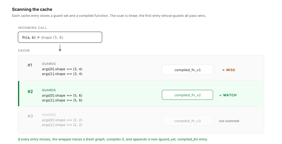
Real Dynamo makes the same trade-off:
| First call | Subsequent calls (cache hit) | Shape change (cache miss) | |
|---|---|---|---|
| Cost | Full trace + compile | Guard checks only | Full retrace + compile |
| Typical time | Milliseconds | Microseconds | Milliseconds |
9. The compile() Decorator
The top-level API ties together all five pipeline stages. The snippet below strips the decorator down to the cache loop; mini_dynamo/__init__.py also handles @compile(backend="jit"), validates the backend name, and rejects non-tensor runtime arguments:
def compile(fn=None, *, backend="python"):
    # The cache lives in this closure, so each @compile'd function gets its
    # own. Entries are appended in the order they were compiled; we scan
    # from the front on every call.
    cache = []

    @functools.wraps(fn)
    def wrapper(*args):
        if not all(isinstance(arg, torch.Tensor) for arg in args):
            raise TypeError("mini_dynamo.compile only supports tensor arguments")

        # Fast path: walk the cache and run the first entry whose guards
        # all pass on the current args. This is the path every steady-state
        # call takes.
        for guard_set, compiled_fn in cache:
            if guard_set.check_all(*args):
                return compiled_fn(*args)       # Cache hit → fast path

        # Slow path: nothing in the cache matches, so run the full pipeline
        # and append a new entry. The next call with the same signature
        # will hit it in the loop above.
        graph = SymbolicInterpreter(fn, args).run()         # STEP 1: Trace
        compiled_fn, _ = compile_graph(graph)                # STEP 2: Compile
        guard_set = GuardSet.from_example_inputs(args)       # STEP 3: Guard
        cache.append((guard_set, compiled_fn))               # STEP 4: Cache
        return compiled_fn(*args)                            # STEP 5: Execute

    # Exposed only so the examples below can inspect the cache and compare
    # against the original eager function.
    wrapper._cache = cache
    wrapper._original = fn
    return wrapper
The previous sections built each component in isolation: the interpreter, the graph, the compiler, and the guards. Now we can run one call through the wrapper and inspect each artifact it produces.
import torch
import mini_dynamo

@mini_dynamo.compile
def fn(x, y):
    z = x + y
    w = z * 2
    return w.sum()

a = torch.randn(3, 4)
b = torch.randn(3, 4)
One reminder from Section 1: the wrapper accepts only positional tensor arguments, and the traced body cannot use keyword calls. Constants like the 2 in x * 2 are fine — they live in the function body and are seen during tracing.
Step 1: Trace
The wrapper’s cache is empty, so we fall into the slow path. SymbolicInterpreter(fn, (a, b)).run() walks fn’s bytecode, pushing VariableTrackers on its stack, and records every tensor operation as a Node. It returns a Graph:
Graph:
  x = placeholder
  y = placeholder
  add_0 = torch.add(x, y)
  mul_0 = torch.mul(add_0, 2)
  sum_0 = mul_0.sum()
  return sum_0
Notice what disappeared: no z = ..., no w = ..., no STORE_FAST noise, no LOAD_GLOBAL torch lookups. The intermediate local variables from the Python source have been flattened into a straight-line DAG of tensor operations. The constant 2 is inlined directly into torch.mul’s args rather than becoming a node. The graph works as an IR because it is a pure description of “what tensor ops, in what order, wired how”, stripped of everything the compiler does not need.
Step 2: Compile
compile_graph(graph) walks those nodes and emits one line of Python per operation. It returns a callable plus the source string, small enough to read in full:
def compiled_fn(x, y):
    add_0 = __fn_add_0(x, y)
    mul_0 = __fn_mul_0(add_0, 2)
    sum_0 = mul_0.sum()
    return sum_0
The __fn_add_0 and __fn_mul_0 names are keys into the namespace the compiler passes to exec(). That dict looks like {"__fn_add_0": torch.add, "__fn_mul_0": torch.mul}, and it becomes the globals for the exec() call that materializes the function. Each op still goes through torch.add and the full PyTorch dispatcher. Each op still launches its own kernel. We have not fused anything, skipped the C++ dispatcher, or avoided a kernel launch.
The Python backend produces a faithful, standalone callable that does what the captured graph says. Kernel fusion and dispatcher elimination happen when you hand the same graph to Inductor instead, which we get to in Section 10.
Step 3: Guard
GuardSet.from_example_inputs((a, b)) inspects each tensor argument and builds three lambda guards per tensor: shape, dtype, and device.
GuardSet([
  args[0].shape == (3, 4)
  args[0].dtype == torch.float32
  args[0].device == cpu
  args[1].shape == (3, 4)
  args[1].dtype == torch.float32
  args[1].device == cpu
])
These six predicates form the contract: “the compiled_fn we just produced is valid as long as these hold”. The guard set is not attached to the tensors a and b; it is a set of checks that future arguments must satisfy.
Step 4: Cache
The pair (guard_set, compiled_fn) gets appended to the cache list. After this first call:
print(len(fn._cache)) # → 1
The cache now has one entry. The cache is per-@compiled function (it lives in the wrapper’s closure), and its order matters. On every later call, we scan it from index 0 upward and return the first entry whose guards all pass.
Step 5: Execute
Finally, we call compiled_fn(a, b) and return the result. The result matches the original eager function. We have reorganized dispatch, not changed the computation:
compiled_fn(a, b) == fn._original(a, b) # → tensor(True)
One first call ran all five steps. The first-call latency (a few milliseconds on our example) is mostly spent in steps 1–3; step 5 takes microseconds.
Second and Third Calls
The structure pays off on later calls. On the second call with the same shape/dtype/device, the wrapper iterates cache, finds that guard_set.check_all(*args) returns True on the first entry, and jumps directly to compiled_fn(*args). Steps 1–4 are skipped entirely. The cache is still length 1.
On the third call with (5, 6) tensors, check_all returns False on every existing entry (the shape guards fail). The wrapper falls through to the slow path again, traces a fresh graph, compiles a new function, builds a new guard set, and appends. Now:
print(len(fn._cache)) # → 2
Future calls scan both entries in order. A (3, 4) call hits entry 0, a (5, 6) call hits entry 1, and any brand-new shape falls through to a new compile and a third entry.
That is the full pipeline in motion. Five stages produce five concrete artifacts: a Graph, a compiled_fn, a GuardSet, a cache list, and a tensor result. Real torch.compile handles more machinery in every stage (keyword arguments, nested calls via PEP 523, dynamic shapes, C-level guard evaluation, per-code-object caches, graph breaks), but the spine has the same shape: trace → compile → guard → cache → execute.
10. Where Does Speedup Come From?
With the full system built, we can ask: how much faster is it?
Graph capture on its own produces no meaningful speedup. The win comes from what an optimizing backend does with the graph. A common description says torch.compile “removes Python overhead.” That phrase bundles together several costs between a user’s x + y and the kernel running on the GPU.
Where the Time Goes
A rough per-op cost decomposition for an elementwise op in eager PyTorch on a modern GPU looks like this. The exact numbers vary by device, driver, PyTorch version, tensor size, and whether you’re on CUDA or MPS, but the ordering is what matters:
| Cost | Typical scale per op | Who pays it |
|---|---|---|
| CPython bytecode dispatch | tens of nanoseconds | The interpreter |
Python-level method resolution, __torch_function__ | hundreds of nanoseconds | CPython + PyTorch’s Python bindings |
| PyTorch C++ dispatcher (device, autograd, vmap, …) | a few microseconds | libtorch |
| Kernel launch onto the CUDA / MPS stream | 5–20 microseconds | The GPU driver |
| The kernel itself | nanoseconds to milliseconds | The GPU |
The first two rows are what most people mean when they say “Python overhead.” They are also the smallest rows. Our Python backend only touches those: it pre-resolves function lookups into the generated function’s namespace so each op skips one LOAD_GLOBAL torch + LOAD_ATTR add pair. Nothing below that line changes. Every op still boxes arguments into PyObjects, still traverses libtorch’s dispatch key logic, still waits on its own kernel launch.
The benchmark numbers follow that pattern, but the exact outcome is backend- and shape-dependent. Running the CPU benchmark examples/benchmark.py on one Slurm node (Python 3.10.12, PyTorch 2.10.0+cu128) produced this 256×256 no-guard result for the raw generated Python function — these are CPU tensors, so Inductor is generating fused C++ kernels here, not GPU code:
Eager (original):             268.9 us
mini_dynamo (python):         267.9 us   (1.00x -- mostly noise)
torch.compile (inductor):      68.0 us   (3.95x)
The CUDA device benchmark needs one subtle precaution: reset Dynamo between per-shape torch.compile runs, otherwise a shape sweep of the same Python function can push Dynamo into a generalized dynamic-shape path and contaminate the later timings. With that reset in place, examples/benchmark_mps.py selected cuda and produced this result on a single NVIDIA H100 80GB:
Tensor size: 2048x2048
Eager:                       160.4 us
mini_dynamo (python):        160.5 us   (1.00x)
mini_dynamo (jit):            33.6 us   (4.78x)
torch.compile (inductor):     30.6 us   (5.25x)
Treat these as measurements of this repository’s toy benchmarks, not universal benchmark results. The stable lesson is narrower and more useful: the Python backend barely moves the needle, the JIT backend can remove Python↔C++ boundary overhead without fusing kernels, and Inductor is the only path here that can change the kernel structure. Whether that structural change wins depends on the operation mix, tensor size, device backend, and PyTorch build.
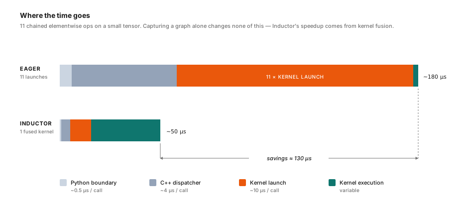
The Python backend’s result is within noise. We saved a handful of bytecodes per op, and the lower layers dwarf that.
The JIT backend’s wins, when they appear, do not come from bytecode dispatch savings. torch.jit.trace wraps the generated function into a single TorchScript graph call, so from Python’s point of view the whole chain becomes one call into C++. Python drops out of the loop between ops, and some of the per-op dispatcher and Python↔C++ boundary-crossing work gets amortized. We’re nibbling at rows 2–3 of the table, not row 1.
Where Inductor Can Win
When Inductor wins, the speedup comes from a different layer. It operates below the dispatcher rather than saving a few interpreter instructions above it, and it relies on having a captured graph as input:
- Kernel fusion. Inductor can generate a single Triton (GPU) or C++ (CPU) kernel for a whole chain of memory-bound ops. Eager does one kernel per operation; for the
many_opsbenchmark above, that means 11 elementwise kernels plus the final reduction. Each kernel reads from HBM, computes one op, and writes back. Fusion reduces those round-trips. For favorable elementwise chains and activations, this often accounts for large speedups in PyTorch benchmarks. - Launch overhead collapse. Even after fusion, each kernel launch still costs microseconds. When the same shapes recur (e.g. the steady-state of a training loop), CUDA graph integration lets you record the launches once and replay them as a single stream op, eliminating the per-step dispatcher and launch costs.
- Memory planning. With a full graph in hand, Inductor can plan intermediate buffers once and reuse them, avoiding the per-op allocator churn eager incurs.
None of these live in our mini-dynamo backend. They require the graph as input, and they operate on the biggest rows of the cost table: the dispatcher, the launch, and the kernel itself. The microseconds live there.
Dynamo Captures, Inductor Optimizes
Dynamo and Inductor solve different problems. Dynamo captures the graph; on its own, that brings almost no performance gain. Inductor optimizes the graph; in many deep-learning workloads, that is where the meaningful speedup comes from. The bytecode tracer exists to hand an optimizing backend a graph it can fuse, schedule, and lower. Our mini-dynamo replaces only the Dynamo part. Because we produce a compatible graph, we can plug in the real Inductor backend and measure the backend’s behavior directly:
We can convert our mini-dynamo graph into an fx.GraphModule, lower it to ATen ops, and pass it directly to compile_fx_inner, Inductor’s internal entry point. This is a private PyTorch API, so the repository pins PyTorch 2.10.0 and treats the integration as educational rather than stable public surface area. For the straight-line tensor programs covered by the parity tests, this produces the same ATen graph as real Dynamo’s export path and the same generated Inductor kernels on the tested backend. The tests validate that narrow claim, not general equivalence across arbitrary PyTorch programs, devices, or Inductor configurations.
def mini_dynamo_to_inductor(fn, *example_inputs):
    # 1. Trace with our symbolic interpreter, producing a mini-dynamo Graph
    #    whose nodes call torch.add, torch.mul, etc.
    graph = SymbolicInterpreter(fn, example_inputs).run()

    # 2. Repackage our graph as a torch.fx.GraphModule, which is the format
    #    Inductor's pipeline accepts.
    gm = to_fx_graph_module(graph)

    # 3. make_fx re-traces gm one more time, this time under PyTorch's ATen
    #    dispatch layer. Surface-level ops (torch.add) get rewritten to their
    #    canonical ATen counterparts (torch.ops.aten.add.Tensor). Inductor
    #    works on ATen, not on the Python-facing torch API.
    aten_gm = make_fx(gm)(*example_inputs)

    # 4. Hand the ATen graph to Inductor's private entry point, which does
    #    the actual kernel fusion and code generation.
    compiled = compile_fx_inner(aten_gm, list(example_inputs))

    # Inductor's callable uses an internal calling convention: it receives
    # one list of tensor inputs and returns a tuple of outputs. Wrap it so the
    # result behaves like the original Python function.
    def wrapper(*args):
        return compiled(list(args))[0]

    return wrapper
11. What We Left Out
Mini-dynamo demonstrates the architecture of TorchDynamo. But real Dynamo is a vastly more complex system. Here are the most important gaps:
PEP 523 Frame Evaluation
Real Dynamo doesn’t use dis.get_instructions(). It installs a C-level frame evaluator via PEP 523 that intercepts every Python frame before CPython’s interpreter runs it — no change to how you call your functions. On top of that interception, real Dynamo’s tracer supports:
-
Function inlining: When
fn()callshelper(), Dynamo traces into the callee by recursively walking its bytecode (during tracing,helper’s frame never actually runs), capturing a single unified graph. Our bytecode walker only sees the top-level function. -
Graph breaks: When Dynamo hits an unsupported operation (a
print(), an unsupported data structure), it can break the graph by compiling what it has so far, executing the unsupported operation in normal Python, and resuming tracing after. Our interpreter has no graph-break machinery: unsupported bytecodes raiseNotImplementedError, and opaque helper calls are recorded only as ordinary call nodes if the narrow tracing path can represent them.
Control Flow
We skip all jump instructions (JUMP_IF_TRUE, FOR_ITER, etc.). Real Dynamo handles control flow by specializing: if the branch condition is a tensor property known at trace time (like x.shape[0] > 5), it evaluates it and traces only the taken branch, guarding on the condition.
Dynamic Shapes
Our guards require exact shape matches. Real Dynamo supports dynamic shapes – symbolic integers that represent unknown dimensions. This avoids recompilation when batch size changes, at the cost of more complex guard logic and symbolic reasoning.
200+ VariableTracker Subclasses
Our four types cover tensors, constants, torch functions, and tensor methods. Real Dynamo has trackers for lists, dicts, ranges, slices, iterators, nn.Module instances, user-defined classes, closures, generators, and more.
12. Summary
torch.compile is a well-structured pipeline:
- Intercept Python execution at the bytecode level
- Replay each instruction symbolically, recording tensor operations into a graph
- Compile the graph with an optimizing backend
- Guard against changes in input metadata
- Cache the result for fast reuse
The symbolic interpreter is a CPython emulator. The graph is an IR. The compiler is a code generator. The guards are boolean predicates. Each component is small enough to understand in isolation. Together, they explain how torch.compile speeds up PyTorch programs. In this mini implementation, the graph-capture machinery is the educational focus; the large speedups arrive once you pair that captured graph with an optimizing backend like Inductor.
The full source code for mini-dynamo is at github.com/itsdaniele/torchdynamo-mini. Every module is heavily commented and designed to be read linearly.
Appendix: File Map
| File | Purpose |
|---|---|
mini_dynamo/__init__.py | The compile() decorator – ties together all five stages |
mini_dynamo/symbolic_interpreter.py | The bytecode walker – CPython emulator on VariableTrackers |
mini_dynamo/variable_tracker.py | Four symbolic value types |
mini_dynamo/graph.py | The computation graph IR (Node + Graph) |
mini_dynamo/compiler.py | Code generation backends (Python + JIT) |
mini_dynamo/guards.py | Guard creation and checking |
examples/benchmark.py | Performance analysis: where speedup comes from |
examples/benchmark_mps.py | GPU benchmark: Python vs JIT vs Inductor |
examples/benchmark_transformers.py | Transformer-style fusion pattern benchmark |
examples/inductor_integration.py | Plugging into the real Inductor backend |
Enjoy Reading This Article?
Here are some more articles you might like to read next: